Development, proliferation and survival of single cell brokers in simulated populations
Cell proliferation is probably probably the most seen characteristic of a rising cell inhabitants and, throughout each experiment, cells develop, die or progress within the cell cycle till they ultimately attain mitosis, break up and provides rise to daughter cells. In an try to provide artificial cell populations composed of unbiased cell brokers interacting with one another, a easy however versatile process was setup, wherein cell cycle transitions and mitosis rely on a mix of things which bear in mind volumetric development, extracellular signalling and DNA replication. The developed process makes use of a Markov chain strategy to mannequin cell cycle development as a succession of states, broadly associated to cycle phases, the place cells transfer from one state to the following in keeping with chances which rely on a number of inside or exterior components (Fig. 1a). Within the mannequin, throughout G1 part cells might cross a checkpoint and transfer to a G1c state the place cells are dedicated to S part in dependence of present quantity and extracellular signalling offered by serum or different components. Equally, G2-M part transition relies on a mix of present cell quantity and serum sort and focus. Coming into S part relies on genomic DNA being prepared for duplication (rfdDNA), whereas full DNA duplication is required to maneuver to G2 part. Throughout M part, nucleus breakdown and cell elongation consequence into cell duplication. Along with the “foremost loop” phases, G1 cells can briefly exit the cycle by coming into G0 and optionally reenter it by transferring into G1c, influenced by cell quantity, native cell crowding and/or serum sort and focus. When cells are extremely confluent or low serum focus persists, they’ve the next likelihood to endure apoptosis which then results in lower in vitality and demise. Cell demise may be the results of cell harm by bodily occasions, like a scratch, or drug addition to the medium. Broken cells can recuperate from harm or endure demise in keeping with the harm stage. Volumetric cell development is simulated by an exponential mannequin wherein, throughout every time interval (Δt), cell quantity will increase in keeping with
$${V}_{t}={V}_{c}cdot{e}^{alpha Delta t}$$
(1)
the place, Vc is the present quantity and α is the expansion charge, which in flip relies on cell sort and cycle part and varies over time and amongst cells, which can develop sooner or slower than the inhabitants common. The described process works successfully with time intervals ranging between a couple of minutes and some hours, in keeping with the necessity. An instance inhabitants, simulated with this mannequin and adopted for 3 days at 20 min time interval, is proven in Fig. 1b–d. The variety of cells (Fig. 1b) exponentially will increase over time, with a median replication time of about 24 h and a small portion of cells present process apoptosis and demise. The accuracy of the replication time obtained by simulating cell cycle on this means was examined by evaluating requested versus calculated replication time (common cell age at mitosis) in a panel of simulated populations (Supplementary Desk 1): for all of them, the 2 values turned out to be at all times very shut, even with a broad vary of replication instances (20–32 h); the obvious duplication time of the identical populations can also be coherent with the expectations as it’s essentially bigger because of the fraction of cells which die or spend time in G0 earlier than present process apoptosis.

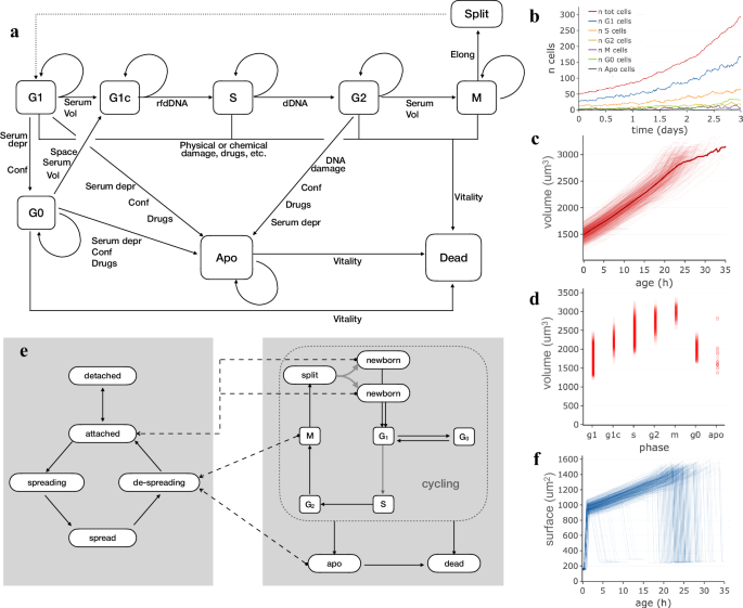
Markov fashions utilized in simulating cell attachment and proliferation and cell inhabitants produced by way of them. a Schema of states and transitions used to simulate part modifications and cell replication. b Development of a simulated inhabitants with common duplication time of 24 h wherein cells are duplicated in keeping with the Markov chain primarily based cell cycle mannequin; the completely different strains report the variety of cells within the completely different cycle phases over time. c Cell quantity plotted as a operate of cell age. Every line corresponds to one of many simulated cells within the inhabitants. The thicker curve represents the common quantity. d Cell quantity values in several cycle phases; circles correspond to particular person cells at a given time. e The succession of states used to mannequin attachment and spreading to the plate substratum. Dashed arrows point out part modifications within the cell cycle which produce pressured modifications in attachment state. f Cell floor plotted, individually for every cell, as a operate of cell age.
Cell cycle part composition, as needs to be anticipated, displays part durations and is maintained over time: most cells (50–60%) are in G1, 20–30% of cells are in S part, whereas smaller fractions of cells are within the different phases (Fig. 1b). Cell quantity, plotted as a operate of age individually for every cell (Fig. 1c), exhibits an total improve sample though, throughout the similar inhabitants, curves differ for various cells as inside state and exterior components play a job in producing variability between cells. Cell quantity modifications through the cell cycle (Fig. 1d), progressively rising from G1 to M part. Cell numbers and volumes, calculated in keeping with this mannequin, are coherent with identified doubling instances and never removed from development patterns experimentally noticed in several cell cycle phases48,49,50,51,52.
Cells rising on a tradition dish change form and attachment standing following interactions with the substrate and in relation to part modifications. To characterize the affiliation between these processes, a second Markov chain was launched and related to the above described cell cycle mannequin (Fig. 1e). Mainly, a indifferent cell is modelled as freely fluctuating into the medium and has a variable likelihood, relying on substratum and cell sort options, of creating a primary secure contact with the plate thus changing into hooked up. Equally, an hooked up cell has a given likelihood of beginning a spreading course of, thus changing into spreading, i.e. a state wherein it reshapes by progressively flattening its quantity and rising its floor, till it turns into absolutely unfold. Some part modifications within the cell cycle produce modifications in attachment state, represented in Fig. 1e by dashed strains connecting, for instance, M part or apoptosis (apo) state with the de-spreading state. These attachment states can affect cell behaviour by appearing on development charges and motility and could also be used as hints when graphically representing cells. In Fig. 1f, cell floor, plotted as a operate of age for every cell of the beforehand described inhabitants, is proven to quickly improve within the first few hours, because of cell spreading; after that, floor will increase following quantity improve and at last decreases, quickly when cells endure mitosis or extra slowly when de-spreading throughout apoptosis.
In Fig. 2a, two populations of NIH3T3-like simulated cells had been adopted for 15 days whereas rising at serum concentrations of both 10% or 2.5% calf serum along with a 3rd one first rising at 10% and later at 2.5%, after a serum step down on the sixth day. The simulated populations present completely different development charges for the 2 serum concentrations, and cease rising at completely different cell densities when the cultures arrive at confluence and cell numbers change into secure; these patterns are similar to these noticed a very long time in the past in experimental cultures53; see Supplementary Fig. 1 for a graphic comparability. Persistently, the distribution of cells within the completely different cell cycle phases modifications with time: on the third day (exponential development), about half cells are in G1 part at 10% cs, however solely 20% of cells are in G0; the G0 fraction is far greater (52%) in cells rising at 2.5% cs (Fig. 2b). This distinction turns into a lot smaller when populations attain confluence and cell numbers cease rising: beneath these circumstances, cell cycle part composition could be very related for the three analysed populations (fifteenth day). These fractions are very near these noticed beneath related circumstances in experimental cell populations54,55,56,57; for cells exponentially rising at 10% serum, for instance, Kues et al. report 67–73% cells in G0/G1 and 9–16% in S part. In Fig. 2c, d simulated NIH3T3-like cells, seeded at 4 completely different densities, had been “grown” for 15 days at 5% cs. Through the earlier days, the noticed proportion of G0 cells varies and progressively will increase as cell numbers go up, however when, later within the experiment, the stationary part is reached, most cells (~70%) are in G0 part and cell numbers change into unbiased of the preliminary seeding density (Fig. 2c, d).

a Development curve, expressed as variety of cells per 0.58 mm2, obtained for 2 simulated NIH3T3 populations adopted for 15 days whereas rising at 10% (gray) and a couple of.5% (blue) calf serum, and for a 3rd inhabitants (inexperienced) initially saved at 10 calf serum and moved to 2.5% on the sixth day (arrow). b Cell fractions within the completely different cycle phases on the third day (exponential development) and on the fifteenth day (stationary state). c Development curve, expressed as variety of cells per 0.58 mm2, for 4 simulated NIH3T3 populations seeded at 4 completely different densities (1, 4, 10, 50 per 0.58 mm2) and adopted for 15 days whereas rising at 5% calf serum (gray). d Proportion of cells within the completely different cycle phases on the third and fifteenth day. e Development arrest of simulated inhabitants induced by serum hunger and rescue by serum re-addition. NIH3T3-like cells had been simulated whereas rising beneath 10% FBS and, at day 1, starved by transferring them to 0.5% FBS; on day 4 serum was restored to 10% and cells had been adopted for 3 extra days. Complete variety of cells (blue line) and the variety of cells in S (inexperienced line) and G0 (yellow line) part are proven within the plot. f Snapshots of the simulated inhabitants in (e) at day 1, 3, 5 and seven are reported by plotting every cell in keeping with cdt1 and p27 focus.
Cells simulated on this means reply to completely different ranges of serum by modifying their development charge and development by way of the cell cycle; their behaviour beneath extra excessive circumstances was examined to see whether or not they react by momentary or completely arresting cell cycle development. In Fig. 2e, NIH3T3-like cells had been simulated initially as rising beneath 10% FBS after which as starved by lowering FBS to 0.5%; outcomes present that whereas cells are saved at 10% FBS, they exponentially develop over time however, when starved by stepping down FBS to 0.5%, cells decelerate till they cease rising in quantity as a big fraction (79–85%) of cells enter G0 part, a fraction very near the 78–80% noticed in experimental populations beneath related circumstances47. Cell rescue from hunger, by once more elevating FBS to 10%, causes cells to enter S part and synchronously restart development and proliferation till they attain confluence and decelerate once more. With a purpose to monitor cell cycle modifications, the buildup of two reporter proteins, cdt1 and p27, steadily used as markers for G1 and G0, respectively, was additionally simulated by relating their synthesis to intracellular state and propensity to part modifications. In Fig. 2f, the place every simulated cell is positioned within the plot in keeping with the focus of the 2 proteins on the indicated day, for every of the completely different serum ranges the outcomes are per curves in Fig. 2e and similar to these reported within the literature for a similar cell sort beneath related circumstances55,56. Cells “grown” beneath 10% FBS (day1) largely have low p27 ranges, following a sample typical of biking cells, whereas cells saved in low serum largely present excessive ranges of each cdt1 and p27, a sample typical of G0 part (day3). Cells rescued by elevating serum again to 10% step by step reenter cell cycle as confirmed by the diminished p27 ranges (day5) which once more go up on the seventh day once they begin reaching confluence. Supplementary Determine 2 represents the identical plots, utilizing color to spotlight the part of each single cell: within the overwhelming majority of instances, the amount of p27/cdt1 matches the cell cycle part.
Cell movement paths generated in silico precisely reproduce experimental cells transferring on a tradition floor
Simulation of cell motion was setup by profiting from a beforehand revealed movement mannequin, which describes motion of experimental cell populations as the mix of three vectors: a random, a persistence and a directional bias element47. The process, reported in Fig. 3a and within the Strategies part, makes use of random, bias and/or persistence vectors to provide migration paths equivalent to utterly diffusive, persistent or directionally biased actions, in numerous combos. For every time interval, remaining cell displacement (d) is simulated by combining a random vector (r) with a persistence one (p), characterised by a person outlined module and the identical course because the earlier cell displacement (prev d), and a person outlined exterior bias vector (b). Whereas the mix of purely random displacement steps produces a comparatively tortuous “Random path”, the “Blended path” generated by extra advanced motion varieties can also be characterised by directional persistence and/or bias alongside a given angle. The paths adopted by two simulated populations, respectively characterised by “Random” and “Blended” motion, are reported within the left column of Fig. 3b; in each instances, particular person paths are completely different from one another and reproduce the variability sometimes noticed in experimental cell cultures. Purely random paths, analysed in keeping with the three-component mannequin, present a 8.7 µm random module whereas persistence and bias ones are very near zero; displacement lengths (centre column) present a long-tailed distribution peaking across the random module, with randomly distributed instructions. Density distribution of displacement endpoints, plotted as ranging from the origin (proper column), exhibits the best frequencies (indicated by hotter colors) across the origin and uniformly enlarges in all instructions. Blended motion, simulated by including a persistence and a bias vector, produced extra linear paths, directed in the direction of the bias angle (0°), with estimated persistence and bias modules of about 4 µm. Accordingly, displacement instructions are clustered across the bias angle whereas modules are greater than in random paths though nonetheless displaying a long-tailed distribution. Cell displacements are strongly shifted within the course of the bias vector however stay symmetrically distributed across the x axis. When simulated cell displacements are adopted over time (Fig. 3c), their distribution progressively enlarge in all instructions with time, sustaining the best frequencies across the origin for random actions, and shifting it in the direction of the bias course for combined inhabitants.

a Simulation of single cell displacement and full paths. The highest schema exhibits the development of a cell displacement (d), produced by combining a random vector (r) with a persistence one (p), characterised by a person outlined module and the identical course because the earlier cell displacement (prev d), and an exterior bias vector (b) alongside person outlined course. The decrease two schemas report examples of a purely “Random” path and a “Blended” one, wherein directional persistence and bias have been added. b Paths and displacements produced by simulating two cell populations characterised by “Random” (prime row) or “Blended” (backside row) motion. For every simulated inhabitants, the paths adopted by every cell are reported within the left column, with, under every graph, the values of random, persistence and bias modules obtained by analysing them by utilizing the three-component mannequin47; an opacity gradient is used to mark the passing of time whereas drawing cell paths. Within the center column, displacement modules are reported as a operate of course, with their distributions reported as histograms alongside the 2 axes. The suitable column experiences, for every cell inhabitants, cell displacements as two-dimensional kernel density distribution of shifts from earlier positions utilizing a color code (heat to chilly colors correspond to greater to decrease density areas); a tridimensional illustration of the identical knowledge can also be included. c For every cells inhabitants, the identical two-dimensional kernel density distribution is reported utilizing shifts equivalent to 4 completely different time intervals, 40, 80, 120, 160 min.
With a purpose to take a look at the flexibility of the described process to breed the conduct of experimental cell populations noticed in time-lapse experiments, the three-component mannequin was used to calculate, from a panel of experimental cell cultures, random, persistence, and directional parts for use to generate motion in simulated populations. The panel consists of plenty of human tumour-derived cell strains (HeLa, T24, MDA-MB-231, PC3, A2058, A375, Calu and wm115) in addition to two strains from murine embryonal fibroblasts, NIH-3T3 and NIH-Ras, the latter over-expressing a constitutively lively variant of Ras, additionally identified to be current in T24 cells. All strains had been cultured and analysed whereas exponentially rising beneath normal circumstances; for HeLa, T24 and NIH-3T3 strains, movement parameters had been additionally decided whereas cells had been transferring in wound therapeutic assay for 12 h after scratching the cell layer (Supplementary Desk 2). Random, persistence and bias modules from experimental HeLa, T24 and NIH-3T3 populations had been used to simulate movement behaviour of a small inhabitants of the identical dimension because the experimental one, in addition to a regular 50 cell inhabitants (Desk 1). The outcomes present very related values for random, bias and persistence parts for all populations of the identical group and are nicely separated from these of the opposite teams (Supplementary Determine 3). Apparently, simulated populations are very near experimental ones additionally for extra motion parameters, not used to generate the simulated populations, akin to common displacement module, remaining MSD and rMSD (random Imply Squared Displacement). As well as, simulations had been additionally capable of match the superdiffusive movement parameter α, constantly near these obtained from the experimental populations and in addition greater when cells transfer responding to wound stimulus. On this case, persistence time, linearity and coherence in addition to round statistics R parameter additionally present correspondingly greater values. Paths generated by simulating normal populations additionally seem similar to these initially noticed within the experimental cultures (Fig. 4a). As well as, simulations reproduce many options of the experimental populations and keep the variations between cell strains, with tortuous paths for HeLa, extra linear and protracted ones for T24 and intermediate options for NIH-3T3 cells. Cells simulated whereas transferring in the direction of the wound produced directionally biased actions, related each in look and as estimated parameters (Fig. 4b). Lastly, in Fig. 4c, the variability of various simulated populations, generated from the identical configuration parameters, was examined by producing, for every experimental inhabitants, ten simulated ones with the identical variety of beginning cells and ten extra with 50 beginning cells every. For every of 11 parameters measured in each experimental and simulated populations, the distributions of values obtained from every group of simulated populations are displayed as field and whiskers plot alongside the corresponding values obtained from the experimental populations. The obtained distributions had been relatively tight for all examined parameters, even in populations characterised by decrease cell numbers, and values from experimental cultures largely fall inside, or are very near them. Extra variable values had been solely noticed for diffusion coefficient and persistence time: additionally on this case the bigger distributions noticed in small populations change into tighter when bigger numbers of beginning cells are used. It’s price noting that solely three of the eleven parameters had been used to configure the simulated populations (grey-background plots). Though not associated to motion, replication time was additionally decided for a similar populations with outcomes reported in Supplementary Fig. 4: additionally on this case, the obtained distributions had been relatively tight and values from experimental cultures fall nicely inside them.

For HeLa, T24 and NIH-3T3 populations, x–y coordinates registered throughout experimental time-lapse acquisitions and simulation experiments had been used to attract paths adopted by every cell, each beneath normal tradition circumstances (a) and through wound therapeutic experiments (b); an opacity gradient is used to mark the passing of time whereas drawing cell paths. The calculated random (r), persistence (p) and bias (b) modules had been reported beneath every graph. c For each normal and wound circumstances, 10 populations had been simulated beginning both with the identical variety of cells as within the corresponding experimental one (purple packing containers) or with a regular variety of 50 cells (blue packing containers): for every motion parameter, a plot experiences the distribution of its values among the many simulated populations in contrast with the worth obtained from the corresponding experimental one (black dashes). A gray background within the plot signifies parameters used to configure the options of the simulated cell populations.
From reproducing cell subpopulations to predicting conditional cell behaviour on a tradition plate
Not like the earlier simulations, the place populations or subpopulations are homogenous and cell-to-cell variations largely derive from apparently random particular person variability, the behaviour of various cells rising on a tradition dish is extra seemingly not homogenous and modifications in keeping with intracellular state and/or native exterior circumstances, thus giving rise to a doubtlessly giant variety of completely different subpopulations throughout the similar tradition. To breed this cell-by-cell variability, the above-described movement mannequin was prolonged to incorporate the flexibility to change pace, directionality, and different options in keeping with the presence of an attractant, repulsion from neighboring cells, attachment state, and cell cycle part. The strategy for producing motion was due to this fact modified to bear in mind the various components capable of modify motion, whereas calculating the displacement of every particular person cell (Fig. 5a). Mainly, random (rand), persistence (pers) and bias (bias) modules, obtained from an experimental inhabitants, had been respectively assumed to be the results of the next expressions:
$${rand}=rcdot{d}_{{tot}}$$
(2)
$${pers}=pcdot{d}_{{tot}}$$
(3)
$${bias}=bcdot{d}_{{tot}}$$
(4)
the place r, p, b, whose sum is the same as one, correspond to the fraction respectively utilized by random, persistence and bias parts of dtot, i.e. the “most potential displacement” of a given cell sort, travelling beneath a given situation. The common dtot worth noticed within the experimental inhabitants is in flip assumed to derive from a reference worth, dref, by way of a coefficient okay, representing the cumulative impact of cell confluence, restricted vitamins or development issue availability, or different inhibitors of cell motion. When producing motion with the prolonged movement mannequin, for every simulated cell, dtot is re-calculated by multiplying dref for a okay worth relying on numerous components together with cell cycle part, attachment state, stage of vitality and native confluence. Equally, b is modified by making an allowance for the impact of things capable of affect the ultimate bias vector, akin to international bias, repulsion from neighbouring cells or bias because of the presence of an attractant gradient. Re-calculated r, p, b and dtot at the moment are used to acquire the brand new random, persistence and bias modules, which, mixed in keeping with the three element mannequin, give the ultimate displacement. Lastly, cell place is modified utilizing the obtained displacement and optionally making an allowance for the presence on the tradition floor of bodily borders or different constraints which decelerate or utterly block cell motion.

a The prolonged movement mannequin used within the simulator builds on the unique three element mannequin, contained within the dashed field, to simulate the affect of inside and exterior components on cell motion. dtot is the utmost displacement for an outlined time interval and is derived from dref, assumed to be the utmost potential displacement obtained for a similar cell sort beneath an “optimum” set of circumstances; r, p and b point out how a lot of dtot is critical to provide the corresponding random, persistent and bias parts. By modifying these parameters, a variety of things can affect cell displacement and its remaining place; examples are cell cycle part, attachment state, stage of vitality and of native confluence, the presence of bodily constraints and “native” bias, like repulsion from neighbouring cell or attraction because of the presence of an attractant gradient within the plate. b Cell-cell repulsion gradient represented as color shades equivalent to cell affect on the encompassing setting. For every cell, the repulsion vector is reported as a white arrow alongside the straight line between two neighbouring cells and whose module relies on gradient. The time interval between the primary three photographs was 20’ intervals, whereas the others had been taken at 10’ interval. c Impact of a comparatively sharp attractant gradient on cell motion. For every cell, the bias vector is reported as an arrow whose module relies on the distinction in attractant stage over a distance equivalent to the scale of the cell physique. d Impact of dynamic self-generated native gradients on cell motion. The bias vector is reported as an arrow with a module which, as in c, relies on attractants stage, which, on this case, is regionally modified by the presence of cells capable of degrade the attractant molecule in its instantly neighborhood: greater cell focus produces better gradient than sparse cells. In each panels, a extra intense blue signifies greater attractant stage.
As with the prolonged movement mannequin it’s comparatively straightforward to compose the results of various components concurrently affecting the motion of each single cell, assist was added for brief vary cell–cell repulsion and regionally variable gradients of attractant molecules.
Cell-cell repulsion was decided by figuring out, for a given cell, the neighbouring cells inside a given distance and by calculating, for every of them, a repulsion vector alongside the straight line between the 2 cells with a module relying on distance, cell pace and sensibility to repulsion by different cells (Fig. 5b).
Equally, to simulate the impact of gradients of attractant molecules, one other bias vector is set from the distinction in attractant stage between back and front of a given cell. This vector works very properly for brief and/or sharp gradients capable of produce focus variations at distances akin to the scale of a cell physique (Fig. 5c). Assist for shallow gradients was launched by contemplating the impact of dynamic self-generated native gradients as these beforehand described in literature58,59, which assume {that a} shallow and even utterly flat gradient is regionally bolstered by the flexibility of cells to degrade the attractant molecule of their instantly neighborhood (Fig. 5d). Such native gradients have been proven by completely different authors to be extra sturdy, to work throughout better distances and to be higher suited to characterize the impact of the native setting than purely passive cell responses60,61,62,63,64,65,66.
The prolonged movement mannequin can successfully generate, as proven in Fig. 6, the number of completely different cell subpopulations typical of wound therapeutic experiments, ranging from the parameters decided from an experimental NIH-3T3 tradition exponentially rising beneath normal circumstances and transferring in absence of any directional bias. As proven in Fig. 6a, the unique experimental tradition (left panels) was analysed to acquire the “base parameters” r, p, b and dref, which had been then used to provide a equally numbered inhabitants of simulated cells (proper panels) which, “rising” beneath the identical circumstances, attain a comparable variety of cells in 24 h and, on the similar time, transfer alongside related paths (Fig. 6b). The contributions to displacement of the three parts, evaluated over time (see Strategies), present a sample much like the experimental inhabitants, with a median displacement largely product of a random element, with a smaller persistence and no bias (Fig. 6c). In Fig. 6d, the identical “base parameters” had been used to simulate a wound therapeutic experiment the place cells are grown at excessive density, to make them initially produce an extremely confluent “layer” which is then subjected to a scratch. Whereas “rising” at excessive density, dtot values are diminished by decrease nutrient availability or particular mobile states: for instance, cells transfer slower when in G0 or throughout apoptosis. After the scratch, cells by themselves have a tendency to maneuver in the direction of the free house by diffusion bolstered by cell-cell repulsion. The “attraction” by the wound was simulated by including two additional parts, each simulated utilizing dynamic self-generated native gradients, which replicate the impact of free house and the attraction by cell particles produced within the wound space quickly after the scratch. The primary makes use of a flat long-lived attractant uniformly current within the plate to characterize the impact of various serum components; the second, with a comparatively brief half-life, simulates the results of molecules launched by scratch broken cells67,68,69,70,71,72,73. The 2 gradients produce two bias vectors which, mixed with others, akin to that launched by cell to cell repulsion, lead to a remaining bias, completely different for every cell. The ensuing behaviour is far more advanced than within the beginning inhabitants and results in wound closure (Fig. 6d, proper panels) with timing and patterns similar to these of an experimental NIH-3T3 inhabitants noticed beneath the identical circumstances (Fig. 6d, left panels). Simulated cell paths present a progressive lower in size and linearity as the gap from wound entrance will increase (Fig. 6e–g) and entrance (fr), center (md) and inside (in) subpopulations, individually analysed produce outcomes which intently resemble these from experimental cultures. The contributions to displacement of the three parts, evaluated over time, additionally present patterns near these of experimental populations, with longer displacements for entrance populations largely as a result of greater bias, a lot decrease displacement and bias values for inside cells with intermediate values for center cells (Fig. 6h). When motion parameters obtained from the evaluation of the simulated populations are in comparison with a bigger variety of experimental populations in the identical circumstances, whole displacement in addition to random, persistence and bias parts are inside or very near the vary of experimental values (Fig. 6i).

Motion parameters obtained from the experimental cell inhabitants, saved beneath normal circumstances, of panels (a-c) had been used to provide artificial populations transferring in a wound therapeutic experiment in panels (d–h). a Part distinction photographs taken at 24 hour distance of cells exponentially rising beneath normal tradition circumstances and in absence of any directional bias (left facet photographs), in comparison with a simulated cell tradition “grown” beneath the identical circumstances and rendered on the similar instances utilizing a phase-contrast impressed symbolic illustration (proper facet photographs). b Motion paths of experimental and simulated cells through the 24 h interval, drawn by utilizing an opacity gradient to mark the passing of time. c Contributions to cell displacement of random (blue), persistence (inexperienced) and bias (purple) evaluated for experimental and simulated cells by analysing, at every time level, overlapping 12-h home windows. d A wound therapeutic simulation, the place the cell inhabitants makes use of parameters from the experimental inhabitants of panel (a), is in comparison with a wound therapeutic experiment that includes an unbiased experimental inhabitants. For each simulated and experimental populations the photographs are organised as in panel (a). e–g Motion paths for experimental and simulated sub-populations equivalent to cells positioned after the wound on the entrance (e), center (f) or again (g), drawn, as in (b), by utilizing an opacity gradient to mark the passing of time. h Common contributions to cell displacement of random (blue), persistence (inexperienced) and bias (purple) evaluated over time, by individually analysing overlapping 12-h home windows for experimental and simulated cells positioned on the entrance (fr), center (md) and again (in). i Distribution of displacement, random, persistence and bias values obtained for experimental cells from 5 populations beneath normal tradition circumstances (purple packing containers), 16 populations on the wound entrance (blue packing containers) and 6 intermediate (inexperienced packing containers) and inside populations (violet packing containers). The corresponding values from the simulated populations are reported as dashes.
Establishing and executing simulations inside SimulCell net utility
The described fashions and procedures can be utilized collectively to provide simulated populations inside SimulCell, an internet utility designed to setup and run simulation experiments and to shortly analyse the outcomes. Enter knowledge might be manipulated utilizing normal dialog packing containers, organised in sections containing experiment, plate, cell and occasion parameters (Fig. 7a). Through the calculation, the appliance gives assist for monitoring the method, by displaying photographs of the simulated cultures and plots reporting variety of cells or different knowledge. After the calculation, the consequence web page shows main parameters and statistics organised in several tables: Historical past, containing abstract outcomes for every time level, Path and Body, the place knowledge are respectively organised by cell and time interval, along with Setup and Efficiency, containing the foremost simulation parameters used to setup the experiment and run period and different efficiency indicators. Nonetheless inside SimulCell, many alternative plots might be generated to visualise knowledge as customized graphs designed to spotlight particular knowledge options (Fig. 7b) and pictures and movies are used to show cell behaviour and morphology through the simulated experiment. Inside SimulCell, as additionally in photographs proven in Fig. 6, cell visualisation makes use of a “symbolic” illustration, the place cells are easy geometric shapes, which change relying on cell sort, standing and situation. Cell physique is represented by a circle or an ellipse whose dimension conveys details about quantity, diploma of spreading and cell polarisation. Pictures use a gray stage color set, harking back to part distinction microscopy, to let the person recognise cell development, attachment standing, nuclear duplication and division in a well-recognized means; some examples are reported in Fig. 7c.

a The setup web page is used to outline a multi-experiment run utilizing the accessible plates, cells and occasions and offers entry to all parameters wanted to run a simulation by way of dialog sections customised for plate, cell and occasion. b The consequence web page provides entry to the simulation outcomes utilizing customised tables and plots and displaying movies to show cell behaviour. c Simulated “symbolic” representations of cell morphology in comparison with part distinction photographs of experimental NIH3T3 cells beneath related circumstances: cells are visualised as oval shapes, whose dimension and elongation rely on cell options in addition to simulated quantity and diploma of spreading; as for his or her experimental counterpart, border color is dimmer in absolutely unfold cells and turns into thicker and clearer when cells de-spread throughout nuclear duplication and division or apoptosis.
Determine 8 exhibits some simulations executed inside SimulCell, which spotlight how cell behaviour is affected by the precise circumstances outlined whereas establishing the experiment and every particular person cell agent integrates completely different points of cell behaviour and reacts to native setting modifications produced by different cells or ensuing from exterior bodily or chemical occasions.

a Variety of simulated NIH3T3-like cells whereas responding to an antibiotic added to the medium at time 6 h and adopted for 8 days. b Part-contrast like photographs of the identical inhabitants on days 0, 1, 3 and 6. c Manufacturing of antibiotic-resistant clones by DNA transfection. After transfection with an antibiotic resistance gene at time 0, the variety of whole simulated NIH3T3-like cells (blue line), non-transfected (inexperienced line) and transfected cells (yellow line) is reported over time whereas cells reply to an antibiotic added to the medium at time 6 h. d Part distinction like photographs of the identical inhabitants on days 1, 4, 6 and eight. e–g Manufacturing of foci by overgrowth after transformation by exogenous DNA. The overall variety of cells (blue line) and the variety of cells in S (inexperienced line) and G0 (yellow line) part after transfection with constitutively activated Ras gene at time 12 h and serum step right down to 1% FBS ate time 24 h is reported for non transfected (e) and transfected cells (f). g Part distinction like photographs of the identical inhabitants on days 2, 6, 8 and 10. h Variety of useless (blue line) and contaminated (inexperienced line) simulated VeroE6 cells after an infection with a lytic virus (9 h replication time). i Part distinction like photographs of the identical inhabitants on days 2, 3 and 4.
Within the instance reported in Fig. 8a, b, the vitality of every cell is otherwise affected by an antibiotic drug added to the medium and simulated cells reply by progressively dying till they utterly disappear over time. When the identical cells are “transfected” with an antibiotic resistance gene, some purchase the brand new gene (Fig. 8c, yellow line), change into proof against the antibiotic and develop and proliferate in its presence, producing resistant clones (Fig. 8c, d) (Supplementary Film1).
In Fig. 8e–g, simulated NIH3T3-like cells had been modified by buying a constitutively lively Ras gene by transfection and later moved to 1% FBS (Supplementary Film2). Below these circumstances, cells continue to grow though at a decrease charge due to diminished serum stimulation and, after just a few days, some cells, having acquired the mutated Ras gene, speed up development and produce clonal foci which after some time begin overcoming the encompassing cells (Fig. 8g and Supplementary Fig. 5). The plots present that in low serum non-transfected cells decelerate their development and enter G0 part, not like the few remodeled cells which actively proliferate and in just a few days begin a quick exponential development and change into the predominant cell inhabitants concomitantly with the looks of foci within the tradition.
Lastly Fig. 8h, i, exhibits the impact of infecting simulated cells with a lytic virus (Supplementary Film3). Right here, cell brokers had been configured with parameters from VeroE6 cells and virus an infection was assumed to result in cell lysis in about 9 h and to launch new infective virus particles within the surrounding space. The outcomes present that 24 h after an infection (day 2) the layer continues to be confluent, however that ranging from day 3, a lysis plaque turns into seen and enlarges over time following the few replication cycles equivalent to the sequential waves of an infection attributable to subsequent native releases of latest virus particles.