Exploring results of platelet contractility on the kinetics, thermodynamics, and mechanisms of fibrin clot contraction

Assortment and fractionation of human blood

Blood from wholesome people was drawn by venipuncture. The examine was accepted by the College of Pennsylvania Institutional Assessment Board. The themes have been excluded from the examine if anticoagulants or antiplatelet medicines have been taken inside 2 weeks earlier than drawing of blood. Blood was stabilized with 3.2% trisodium citrate 9:1 by quantity. The citrated blood was used instantly to acquire platelet-rich plasma (PRP) by centrifugation at 200 g for 10 min at room temperature. One portion of PRP was moreover centrifuged at 1000 g for 15 min to settle and focus platelets. The second portion of PRP was centrifuged at 10,000 g for 15 min to take away platelets and procure platelet-free plasma (PFP). The platelet pellets have been re-suspended in PFP to achieve numerous closing platelet counts, specifically about 1,000,000, 450,000 and 100,000 platelets per 1 µl. The platelet depend was measured utilizing an automatic cell counter system ABX Micros 60 (Horiba, Japan).

Experimental dedication of the kinetics and closing extent of clot contraction

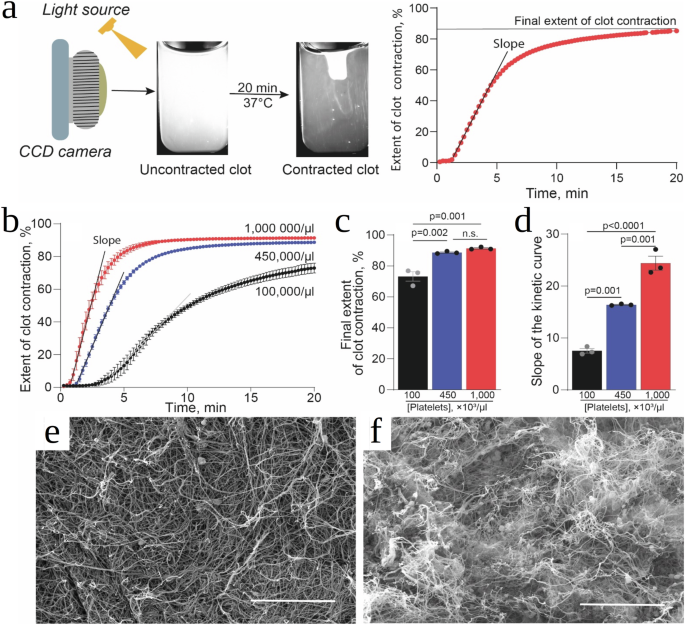
The kinetics of clot contraction have been decided by detecting optically the decreasing clot measurement over time utilizing the Thrombodynamics Analyzer (DiaPharma, USA) principally as described earlier⁸. Prior to make use of, 12 mm × 7 mm × 1 mm clear plastic cuvettes have been lubricated with 1% pluronic F–127 in 150 mM NaCl to stop sticking of the clot to the partitions and permit for the unconstrained clot contraction. To provoke plasma clotting and activate platelets, in a separate plastic tube 2 μl of CaCl₂ (200 mM) and 5 μl or 7.5 μl of freshly thawed human thrombin (40 U/ml) have been added to 200 μl of platelet-containing plasma to achieve a closing focus of two mM CaCl₂ and 1 or 1.5 U/ml thrombin, respectively. 80 μl of the activated plasma pattern was shortly transferred right into a measuring cuvette pre-heated at 37 °C. Imaging of the clot throughout contraction was carried out robotically each 15 s. Digital photographs of the clot have been used to find out the clot measurement at every time level and plot the kinetic curves of contraction/shrinkage till 20 minutes after the addition of thrombin to the pattern, when a plateau was reached.

Scanning electron microscopy of uncontracted and contracted clots

For scanning electron microscopy, PRP clots have been shaped in plastic cylinders 6 mm in diameter. For unconstrained clot contraction, the partitions have been pre-lubricated with 1% pluronic F–127 in 150 mM NaCl to stop sticking of fibrin to the partitions, whereas an uncontracted clot was shaped in a cylinder with a tough interior floor to make sure clot attachment that forestalls contraction. Each the uncontracted and contracted clots have been shaped by including 2 μl of CaCl₂ (200 mM) and seven.5 μl of freshly thawed human thrombin (40 U/ml) to 200 μl of PRP, which was shortly transferred into the corresponding cylinders, and the clots have been allowed to kind for 30 min. The ensuing clots have been washed completely in 50 mM sodium cacodylate buffer containing 100 mM NaCl (pH 7.4) at room temperature, after which mounted in 2% glutaraldehyde in the identical buffer, dehydrated in ascending ethanol concentrations, immersed into hexamethyldisilazane, air-dried, and sputter coated with gold-palladium. The samples have been examined in an FEI Quanta 250FEG scanning electron microscope (FEI, Hillsboro, OR, USA).

Creating digital 3D fibrin clot construction

The preliminary fibrin clot construction utilized in ClotDynaMo had a cubic form (Fig. 2b) 120 µm × 120 µm × 120 µm, with the preliminary quantity ({V}_{0}=) 1.7 × 10⁶ µm³ (different shapes, equivalent to spheres and cylinders, are viable choices). We use the experimental distributions (densities) of the 3- and 4-degree nodes ({rho }_{3}) and ({rho }_{4}) (Supplementary Desk 1) throughout the boundaries of a selected geometry. Every 3-degree (or 4-degree) node connects three (or 4) fibrin fibers. The entire variety of the 3- and 4-degree nodes is given by the components, (N={V}_{0}{rho }_{3}+{V}_{0}{rho }_{4}), and the full variety of fibrin fibers is calculated as (M=frac{3{V}_{0}{rho }_{3}+4{V}_{0}{rho }_{4}}{2}). Subsequent, utilizing the experimental distribution of fibrin fiber lengths (Supplementary Fig. 1), a complete of (M) size values are sampled. For every pair of nodes (i) and (j), the node-to-node distances ({r}_{{ij}}) are calculated and in contrast with (M) values of size generated. Connecting the nodes to kind fibrin fibers satisfies two situations: i) every 3- or 4-degree node has 3 or 4 fibrin fibers, respectively; ii) every fibrin fiber’s size approximates certainly one of (M) size values generated. Given the preliminary random node filling the 3D cubic area, the ensuing histogram of fiber lengths intently (however not precisely) resembles the experimental histogram of fibrin fiber lengths (Supplementary Fig. 1a). To make the simulated distribution of the fibrin fiber lengths to be equal to the experimental distribution, a minimization simulation is carried out, during which every fibrin fiber is represented by a harmonic spring able to growth and contraction. Every fiber’s size steadily relaxes to the equilibrium size, set to be equal to the corresponding worth from the distribution of (M) values of fiber size generated. In consequence, the simulated distribution of the fibrin fiber lengths intently matches the experimental histogram (Supplementary Fig. 1a). Utilizing the same strategy, we regulate the values of fibrin fiber diameters to make the simulated distribution match the experimental histogram of fiber diameters (Supplementary Fig. 1b). To finish the preliminary construction of fibrin fiber community with platelets, the platelets are randomly positioned in proximity to one of many community nodes. The variety of platelets in a clot quantity is calculated primarily based on the goal concentrations (100,000/μl, 450,000/μl or 1,000,000/μl).

Power subject for fibrin clot contraction

Fibrin fibers are described by the stretching potential (({U}_{{fib}}^{{str}})) with the (i)-th cylinder size ({r}_{{fib},i}), the bending potential (({U}_{{fib}}^{{bend}})) with the bending angle between the (i)-th and (i+1)-th cylinders, ({theta }_{{fib},{ij}}), and the excluded quantity interplay potential (({U}_{{fib}}^{{rep}})) between (i)-th and (j)-th fiber cylinders, i.e.

the place ({Okay}_{r}=) 1.15 × 10⁴ nN/µm and ({Okay}_{theta }=) 8.7 × 10⁹ kJ/mol·rad² are the stretching and bending rigidities for fibrin fibers, ({r}_{{fib},0}=) 0.5–12.0 µm is the equilibrium cylinder size (see Supplementary Fig. 1a), and ({theta }_{{fib},0}=) 180° is the equilibrium bending angle. In ({U}_{{fib}}^{{rep}}), (varepsilon =) 2.1 × 10⁵ kJ/mol is the power and ({sigma }_{c}={R}_{i}+{R}_{j}=) 0.1–2.0 µm is the size for the excluded quantity interplay (({R}_{i}) and ({R}_{j}) are the radii of (i)-th and (j)-th cylinders; see Supplementary Fig. 1b), and (uin)[0,1] and (sin)[0,1] are the place components. Platelets’ filopodia: A filopodium is described by the stretching potential (({U}_{p-f}^{{str}})) which is dependent upon the gap between the (i)-th platelet middle and the start of a (okay)-th filopodia ({r}_{p,i-f,okay}), stretching potential (({U}_{f}^{{str}})) for the (okay)-th filopodia with the bead-to-bead distance ({r}_{f,okay}), and the affiliation potential (({U}_{p}^{{ass}})) for the interplay between the (i)-th and (j)-th platelets, i.e.

the place ({Okay}_{p,r}=) 1.45 × 10³ nN/µm is the stretching stiffness, (R=) 1.5 µm is the platelet radius (Supplementary Desk 1), and ({r}_{f,0}=) 2.8 µm is the filopodia size. The (i)–th and (j)–th platelets affiliate if the gap between their facilities ({r}_{p,{ij}}, 1.43 µm. Filopodium-fiber bond: We describe the interactions between filopodia and fibrin fibers utilizing the potentials, which rely upon the distances between the (j)-th filopodium rising finish and the (i)-th fibrin fiber cylinder finish and (i+1)-th fiber cylinder finish, with the distances ({r}_{{fib}-f,{ij}}), ({r}_{{fib}-f,i+1,j}), respectively, and the angles between the filopodium and fibrin fiber cylinder axes ({theta }_{{ij}}), ({theta }_{i+1,j}),

the place ({Okay}_{{att},r}=) 16.7 nN/µm is the stretching stiffness, ({L}_{{fib},i}) is the fiber size, and (alpha in) [0,1]^26,27.

Langevin Dynamics for mechanical elements of fibrin clot contraction mannequin

The dynamic evolution of the mechanical levels of freedom (platelet filopodia, fibrin fibers, and filopodia-fiber linkages) is adopted by numerically integrating the Langevin equations of movement (within the overdamped restrict) for the place ({{boldsymbol{r}}}_{i}) of every mechanical element,

the place (gamma =6pi eta a) is the friction coefficient ((eta) is solvent viscosity and (a) is particle measurement), and ({{boldsymbol{g}}}_{{boldsymbol{i}}}left(tright)) is the Gaussian distributed, zero-average random pressure with the variance ({sigma }^{2}=2{okay}_{B}Tgamma) (({okay}_{B}) is the Boltzmann’s fixed). In Eq. (7), (Uleft({boldsymbol{r}}proper)) is the full mechanical power perform

which defines the deterministic pressure ({F}_{i}=frac{partial Uleft({boldsymbol{r}}proper)}{partial {{boldsymbol{r}}}_{{boldsymbol{i}}}}). The Langevin equations are propagated ahead in time with the time step ({dt}=) 1 µs at room temperature 37 °C ((T=) 310 Okay) utilizing the (eta =) 1.1-cP serum viscosity (Supplementary Desk 2).

Describing kinetics in fibrin clot contraction mannequin

The fibrin community state ({boldsymbol{X}}={{{x}_{j}}}_{{boldsymbol{j}}={boldsymbol{1}}}^{{boldsymbol{J}}}) is specified by the variety of fibers, platelets and platelet-fiber linkages (e.g. filopodia-fibrin attachments) ({x}_{j}) of every kind (j=) 1, 2, …, (J). The time evolution of the likelihood for the community to be in state ({boldsymbol{X}}) is given by (frac{{dP}left({boldsymbol{X}},tright)}{{dt}}=mathop{sum }limits_{mu }^{M}[{alpha }_{mu }({boldsymbol{X}}-{{boldsymbol{S}}}_{{boldsymbol{mu }}})P({boldsymbol{X}}-{{boldsymbol{S}}}_{{boldsymbol{mu }}},t)-{alpha }_{mu }({boldsymbol{X}})P({boldsymbol{X}},t)]), the place ({alpha }_{mu }({boldsymbol{X}})) is the response propensity for the (mu)-th response ((mu =) 1, 2,…, (M)) to happen within the system, and ({{boldsymbol{S}}}_{{boldsymbol{mu }}}) is the (mu)-th column of (Jtimes M) stoichiometry matrix ({boldsymbol{S}}) to explain the adjustments within the variety of molecules when the (mu)-th response happens. The equation above is numerically sampled utilizing the Gillespie strategy, which is predicated on the propensities of chemical reactions^52,53. Briefly, the likelihood that the (mu)-th response will happen throughout the subsequent time interval between (t+tau) and (t+tau +{dt}) is given by ({P}_{0}(t+tau ){c}_{mu }{h}_{mu }{dt}), the place ({P}_{0}(t+tau )) is the likelihood that at time (t+tau) no response has occurred within the earlier time interval. The response propensity for the (mu)-th response is ({alpha }_{mu }={c}_{mu }{h}_{mu }), and the full propensity for all (M) reactions is ({alpha }_{0}=mathop{sum }nolimits_{mu =1}^{M}{alpha }_{mu })^52,53. Examples of response propensity calculation for the filopodium-fibrin affiliation and dissociation reactions are given in SI.

Propensity calculation for the filopodium-fibrin affiliation and dissociation reactions

For a unimolecular response (mu) (e.g., filopodium-fibrin dissociation) to happen with the speed fixed ({okay=okay}_{{off}}), the speed equation for a chemical species of kind (A) (e.g. filopodia-fibrin attachment) is (frac{d{x}_{A}}{{dt}}=-k{x}_{A}). We outline ({c}_{mu }{dt}={cdt}) to be the likelihood {that a} specific mixture of reactants will work together via the identical response (mu) within the time interval ({dt}). If ({h}_{mu }) is the full variety of distinct molecular reactant combos at time (t), then for a single molecule of kind (A), (c=okay) and ({h}_{mu }={x}_{A}), and the response propensity is ({alpha }_{mu }=c{h}_{mu }=okay{x}_{A}). For a filopodium-fibrin fiber affiliation, the speed equation for species ({fib}) (fibrin fiber) and (f) (filopodia) is (frac{d{x}_{{fib}}}{{dt}}=frac{d{x}_{f}}{{dt}}=-k{x}_{{fib}}{x}_{f}), the place ({okay=okay}_{{on}}). If ({h}_{mu }) is the variety of distinct molecular reactant combos for a bimolecular response at time (t), then for a single mixture of ({fib}) and (f), (c=okay/{V}_{0}) and ({h}_{mu }={x}_{{fib}}{x}_{f}), and the response propensity is ({alpha }_{mu }=c{h}_{mu }=okay{x}_{{fib}}{x}_{f}/{V}_{0}). The numerical values for ({okay}_{{on}}) and ({okay}_{{off}}) are given in Supplementary Desk 1.

Calculation of thermodynamic state features for fibrin clot contraction

We used the (sigma) vs. (t) information and the (sigma) vs. (V) diagram (the inset to Fig. 4c), to profile the volume-dependent adjustments within the free power (Delta E), the interior power (Delta U), and the entropy (TDelta S) for the platelet-driven contraction of the fibrin clot. The work carried out on the clot (w) is the same as the free power change (Delta E), i.e. (w=Delta E=Delta U-TDelta S). We carried out numerical integration (from the preliminary clot quantity ({V}_{0}) to the ultimate clot quantity (V)) to calculate the realm below the (sigma)–(V) curve, with the intention to receive the work for fibrin clot contraction, (wleft(Vright)=-{int }_{{V}_{0}}^{V}sigma left({V}^{{prime} }proper)d{V}^{{prime} }), which was then used to generate the profiles of (Delta E) vs. (t) and (Delta E) vs. (V). Utilizing the numerical output, i.e. (Delta U) vs. (t) and (Delta U) vs. (V) information, we generated the profiles (TDelta S) vs. (t) and (TDelta S) vs. (V.)

Numerical implementation

The SRDDM²⁵ was mapped into the ClotDynaMo software program (written in CUDA), with the intention to make the most of an enormous parallelism accessible on Graphics Processing Models (GPUs). Within the Langevin Dynamics, numerical calculation of the non-covalent particle-particle interactions, i.e. the excluded quantity interactions, fiber-fiber interactions leading to formation of cohesive bonds, platelet-platelet interactions and the fibrin fiber-platelet interactions, is the computational bottleneck. But, these interactions are described by the identical mechanical power features (harmonic potentials or Lennard-Jones potentials described by Eqs. (4)-(6)). It’s then doable to execute the identical mathematical operation, e.g., power calculations, analysis of forces, technology of random numbers for calculation of random forces, integration of the equations of movement, for a lot of particles on the similar time. Numerical routines for the technology of (pseudo)random numbers (Hybrid Taos) are described elsewhere^54,55. We applied the particle-based parallelization⁵⁵ for fibrin fiber cylinders and platelet spheres. To hurry up the simulations, we used the neighbor lists with the 20 µm cutoff. These efforts have enabled us to span 15–20 min of the clot contraction time in affordable computational time (few weeks or much less).

Continuum mannequin

Following our research²⁹, we assemble a easy continuum mannequin for isotropic contraction of a fibrin clot utilizing the 8-chain mannequin of polymer elasticity (see SI for extra element)⁵⁶. Within the continuum mannequin, a spherical fibrin clot with traction-free boundaries contracts freely with out constraints. At equilibrium, the clot is stress free. Therefore, the Cauchy stress elements are ({sigma }_{11}={sigma }_{22}={sigma }_{33}=) 0 and the principal stretches are ({lambda }_{1}={lambda }_{2}={lambda }_{3}={lambda }_{* }). By implementing the situation that ({sigma }_{11}={sigma }_{22}={sigma }_{33}=) 0, we receive the next equation (see SI): ({g}^{{prime} }left({lambda }_{* }^{3}proper)=-frac{1}{{lambda }_{* }}frac{nu L}{3{lambda }_{* }}left{{EA}left(1-frac{1}{{lambda }_{* }}proper)+{F}_{p}left(tright)proper}=Kleft({lambda }_{* }^{3}-1right)) which might be re-written as

In Eq. (9), (nu) is the variety of fibers per reference quantity, (L) is the common size of fibers between cross-links (department factors in a fibrin gel), (E) is the Younger’s modulus, (A) is the cross-sectional space of a fiber and (Okay) is a bulk modulus of the fiber community. In Eq. (9), ({F}_{p}(t)) is the energetic pressure exerted on a fiber by platelet filopodia, and Eq. (9) might be solved for ({lambda }_{* }) if ({F}_{p}(t)) is understood. ({F}_{p}(t)) is assumed to rely upon platelet focus per reference quantity (c) and filopodia size (l), and is allowed to vary with time:

In Eq. (10), ({F}_{0}) is the pressure generated by a platelet, (p(c)) and (q(l)) are dimensionless features of platelets depend (c) and filopodia size (l), respectively, and (tau) is a attribute time over which the fibrin clot contraction happens. Within the mannequin, (tau) relies upon solely on the viscosity of the atmosphere (eta). The useful types of (p(c)) and (q(l)) usually are not identified, however they are often obtained by becoming the information from the ClotDynaMo simulations with platelet depend (c=) 450,000/µl. Following Brown et al. ²⁹, we set ({EA}=) 3.87 × 10⁻⁷ N, ({F}_{0}=) 10⁻⁹ N, (Okay=) 1 MPa, and (nu L=) 10¹³ m⁻². The extent of contraction (frac{left({V}_{0}-Vleft(tright)proper)}{{V}_{0}}) is then calculated utilizing the components: (frac{left({V}_{0}-Vleft(tright)proper)}{{V}_{0}}=1-{lambda }_{* }^{3}).

Derivation of the continuum mannequin

Our mannequin is predicated on the 8-chain mannequin for polymer elasticity that was tailored to fibrin gels in Brown et al. ²⁹. This mannequin was efficiently utilized to mannequin the tensile habits of fibrin gels, together with the discount in quantity below uniaxial tensile hundreds. A gorgeous characteristic of the 8-chain mannequin is that it connects the force-stretch relation of particular person polymer chains or fibers to the general stress-strain habits of an isotropic community of those fibers. In Brown et al. ²⁹ the tensile habits of single fibrin fibers was computed first and it then entered the 8-chain mannequin to offer wonderful settlement with the tensile habits of centimeter scale gel specimens. In Ramanujam et al.⁵⁷ a variant of the 8-chain mannequin was used to explain cracked fibrin gel. The important thing to accurately capturing the easy shear habits of fibrin gels on this paper was accounting for the buckling of fibers below compression. To account for buckling of fibers in a easy approach the authors assumed that the force-stretch response in compression was delicate for small strains, but it surely progressively stiffens because the stretch of the fiber turns into smaller and approaches zero. Because the platelet induced contraction of clots entails isotropic compression alongside all instructions on the unit sphere, we will even assume the same force-stretch response of fibrin fibers below compression.

To mannequin the contractile impact of platelets, we assume that an energetic agent sits on the physique middle of the 8-chain dice. This energetic agent exerts forces on all eight fibers rising from the middle of the dice. If the aspect of the dice is held mounted, then then the stress in every fiber attributable to the energetic agent is ({F}_{p}(t)) below isotropic contraction. This pressure is unbiased of the state of deformation of the dice. This can be a key modification to the 8-chain mannequin that may allow us to account for the contraction of clots on account of platelet exercise. We shall be involved with isotropic contraction of clots on this doc though the next evaluation is relevant additionally to different geometries. We are going to comply with the event in Brown et al.²⁹. Within the principal coordinate system, the deformation gradient tensor and the correct Cauchy-Inexperienced tensor are, respectively,

and

the place ({lambda }_{1}), ({lambda }_{2}), ({lambda }_{3}) are the principal stretches. We assume that the 8-chain dice is aligned with the principal instructions. On this case the stretch ({lambda }_{c}) of every fiber within the 8-chain dice is given by:

the place ({I}_{1}) is the hint (or first invariant) of the Cauchy-Inexperienced tensor, ({I}_{1}={rm{Tr}}(C)). ({J}^{2}=det (C)) is the determinant (or third invariant) of the Cauchy-Inexperienced tensor. The pressure power per unit reference quantity of the continuum represented by the 8-chain dice (with no platelets) is given by

Within the above (nu) is the variety of fibers per reference quantity, (L) is the common size of fibers between cross-links (department factors in a fibrin gel), (G({lambda }_{c})) is the Helmholtz free power per reference size of a fiber as a perform of stretch ({lambda }_{c}) and (g(J)) is the dilatational a part of the pressure power density of the continuum. The pressure in a fiber is given by

the place (Fleft({lambda }_{c}proper)=frac{dleft(Gleft({lambda }_{c}proper)proper)}{d{lambda }_{c}}) is the pressure on account of elastic stretching (or contracting) of a fiber and ({F}_{p}(t)) is the (energetic) pressure exerted on a fiber by platelets. The principal elements of the second Piola stress are given by:

The Cauchy stress is given by (sigma =frac{1}{det (F)}{FS}{F}^{T}), so

Having obtained the stresses within the continuum by way of the pressure in a fiber, we now contemplate isotropic contraction of clots. We should assume particular varieties for (F({lambda }_{c})), ({g}^{{prime} }left({lambda }_{1}{lambda }_{2}{lambda }_{3}proper)) and ({F}_{p}left(tright)) to write down equations for the contraction of a clot. We take

the place (E) is the Younger’s modulus and (A) is the cross-sectional space of a fiber. For ({lambda }_{c}=1+{epsilon }_{c})_, the place (left|{epsilon }_{c}proper|ll) 1 the elastic force-stretch relation of the fiber is (F={EA}{epsilon }_{c}), no matter the signal of ({epsilon }_{c}) (i.e. linear force-strain relation for small strains no matter tensile or compressive strains). For ({lambda }_{c},)→ 0 the above force-stretch response is stiffening. Preliminary delicate response for small compressive pressure and a stiffening response for giant compressive pressure is attribute of buckled fibers that come into self-contact in a contracted clot. Subsequent, we assume ({g}^{{prime} }left({lambda }_{1}{lambda }_{2}{lambda }_{3}proper)=Okay({lambda }_{1}{lambda }_{2}{lambda }_{3}-1)) with (Okay=) 1 MPa being a bulk modulus. With these assumptions in place setting ({sigma }_{11}={sigma }_{22}={sigma }_{33}=) 0 results in Eq. (9).

Darcy regulation interpretation of preliminary contraction velocity

Think about a skinny rectangular fibrin clot as utilized in experiments depicted in Fig. 1a. Within the undeformed state (earlier than clot contraction happens), the volume-fraction of a strong element (fibrin fibers plus platelets) is ({phi }_{s}.) The quantity of strong within the contracting clots stays mounted whilst the amount of liquid contained in it adjustments with time (t). In our idealized scenario, we assume that the width of the clot stays mounted and that the underside edge doesn’t transfer whereas the highest edge strikes downwards as platelets exert contractile forces on the fibrin fiber community. The origin of the (z)-axis is positioned on the underside fringe of the clot. The peak (hleft(tright)) of the clot adjustments as a perform of time and the preliminary peak is (hleft(0right)=H.) The liquid flux (Q) within the (z)-direction is given by a Darcy regulation

the place (eta) is liquid (serum) viscosity, (okay) is a Darcy fixed and ({dp}/{dz}) is a hydrostatic strain ((p)) gradient within the (z-) route. The strain within the clot is because of forces exerted by activated platelets. We assume that hydrostatic strain (p) is uniform in a lot of the clot, besides in a area of thickness ({rm{delta }}) close to the highest edge the place a lot of the strain drop happens, in order that (Q=-{kp}/eta delta .) The strain within the clot itself is assumed to be linearly proportional to the pressure via a bulk modulus (B):

Such a relation shall be legitimate when the deformations are small, i.e. within the early phases of clot contraction. Due to this fact, the liquid flux from the highest floor is (Q=-frac{{kB}}{eta delta }left(1-frac{h}{H}proper).) Now, the flux of liquid via the highest edge is simply the amount of the liquid going out via the highest floor per unit time divided by the realm of the highest floor, so flux has the models of velocity. Actually, that is the rate (v) of the fibers relative to the fluid on the prime floor of the clot. We discover that (v) is immediately proportional to the modulus (B) and inversely proportional to the viscosity (eta)⁵⁸.